
Neural Network with MXNet in Five Minutes
This is the first tutorial for new users of the R package mxnet. You will learn to construct a neural network to do regression in 5 minutes.
We will show you how to do classification and regression tasks respectively. The data we use comes from the package mlbench.
Preface
This tutorial is written in Rmarkdown.
- You can directly view the hosted version of the tutorial from MXNet R Document
- You can find the download the Rmarkdown source from here
Classification
First of all, let us load in the data and preprocess it:
require(mlbench)
## Loading required package: mlbench
require(mxnet)
## Loading required package: mxnet
## Loading required package: methods
data(Sonar, package="mlbench")

Sonar[,61] = as.numeric(Sonar[,61])-1
train.ind = c(1:50, 100:150)
train.x = data.matrix(Sonar[train.ind, 1:60])
train.y = Sonar[train.ind, 61]
test.x = data.matrix(Sonar[-train.ind, 1:60])
test.y = Sonar[-train.ind, 61]
Next we are going to use a multi-layer perceptron as our classifier. In mxnet, we have a function called mx.mlp so that users can build a general multi-layer neural network to do classification or regression.
There are several parameters we have to feed to mx.mlp:
- Training data and label.
- Number of hidden nodes in each hidden layers.
- Number of nodes in the output layer.
- Type of the activation.
- Type of the output loss.
- The device to train (GPU or CPU).
- Other parameters for
mx.model.FeedForward.create.
The following code piece is showing a possible usage of mx.mlp:
mx.set.seed(0)
model <- mx.mlp(train.x, train.y, hidden_node=10, out_node=2, out_activation="softmax",
                num.round=20, array.batch.size=15, learning.rate=0.07, momentum=0.9,
                eval.metric=mx.metric.accuracy)
## Auto detect layout of input matrix, use rowmajor..
## Start training with 1 devices
## [1] Train-accuracy=0.488888888888889
## [2] Train-accuracy=0.514285714285714
## [3] Train-accuracy=0.514285714285714
## [4] Train-accuracy=0.514285714285714
## [5] Train-accuracy=0.514285714285714
## [6] Train-accuracy=0.523809523809524
## [7] Train-accuracy=0.619047619047619
## [8] Train-accuracy=0.695238095238095
## [9] Train-accuracy=0.695238095238095
## [10] Train-accuracy=0.761904761904762
## [11] Train-accuracy=0.828571428571429
## [12] Train-accuracy=0.771428571428571
## [13] Train-accuracy=0.742857142857143
## [14] Train-accuracy=0.733333333333333
## [15] Train-accuracy=0.771428571428571
## [16] Train-accuracy=0.847619047619048
## [17] Train-accuracy=0.857142857142857
## [18] Train-accuracy=0.838095238095238
## [19] Train-accuracy=0.838095238095238
## [20] Train-accuracy=0.838095238095238
Note that mx.set.seed is the correct function to control the random process in mxnet. You can see the accuracy in each round during training. It is also easy to make prediction and evaluate.
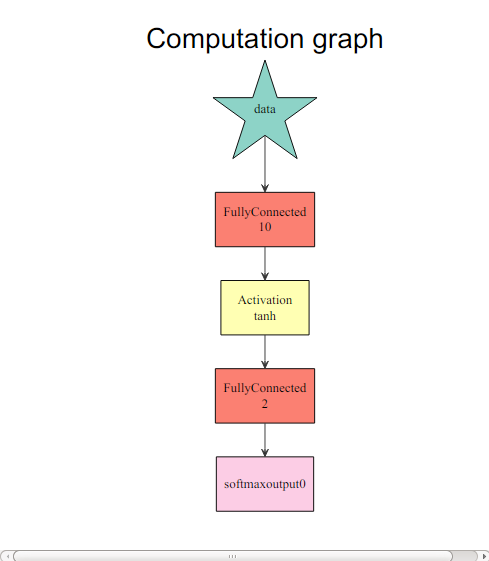
To get an idea of what is happening, we can easily view the computation graph from R.
graph.viz(model$symbol$as.json())
preds = predict(model, test.x)
## Auto detect layout of input matrix, use rowmajor..
pred.label = max.col(t(preds))-1
table(pred.label, test.y)
##           test.y
## pred.label  0  1
##          0 24 14
##          1 36 33
Note for multi-class prediction, mxnet outputs nclass x nexamples, each each row corresponding to probability of that class.
Regression
Again, let us preprocess the data first.
data(BostonHousing, package="mlbench")

train.ind = seq(1, 506, 3)
train.x = data.matrix(BostonHousing[train.ind, -14])
train.y = BostonHousing[train.ind, 14]
test.x = data.matrix(BostonHousing[-train.ind, -14])
test.y = BostonHousing[-train.ind, 14]
Although we can use mx.mlp again to do regression by changing the out_activation, this time we are going to introduce a flexible way to configure neural networks in mxnet. The configuration is done by the “Symbol” system in mxnet, which takes care of the links among nodes, the activation, dropout ratio, etc. To configure a multi-layer neural network, we can do it in the following way:
# Define the input data
data <- mx.symbol.Variable("data")
# A fully connected hidden layer
# data: input source
# num_hidden: number of neurons in this hidden layer
fc1 <- mx.symbol.FullyConnected(data, num_hidden=1)

# Use linear regression for the output layer
lro <- mx.symbol.LinearRegressionOutput(fc1)
What matters for a regression task is mainly the last function, this enables the new network to optimize for squared loss. We can now train on this simple data set. In this configuration, we dropped the hidden layer so the input layer is directly connected to the output layer.
next we can make prediction with this structure and other parameters with mx.model.FeedForward.create:
mx.set.seed(0)
model <- mx.model.FeedForward.create(lro, X=train.x, y=train.y,
                                     ctx=mx.cpu(), num.round=50, array.batch.size=20,
                                     learning.rate=2e-6, momentum=0.9, eval.metric=mx.metric.rmse)
## Auto detect layout of input matrix, use rowmajor..
## Start training with 1 devices
## [1] Train-rmse=16.063282524034
## [2] Train-rmse=12.2792375712573
## [3] Train-rmse=11.1984634005885
## [4] Train-rmse=10.2645236892904
## [5] Train-rmse=9.49711005504284
## [6] Train-rmse=9.07733734175182
## [7] Train-rmse=9.07884450847991
## [8] Train-rmse=9.10463850277417
## [9] Train-rmse=9.03977049028532
## [10] Train-rmse=8.96870685004475
## [11] Train-rmse=8.93113287361574
## [12] Train-rmse=8.89937257821847
## [13] Train-rmse=8.87182096922953
## [14] Train-rmse=8.84476075083586
## [15] Train-rmse=8.81464673014974
## [16] Train-rmse=8.78672567900196
## [17] Train-rmse=8.76265872846474
## [18] Train-rmse=8.73946101419974
## [19] Train-rmse=8.71651926303267
## [20] Train-rmse=8.69457600919277
## [21] Train-rmse=8.67354928674563
## [22] Train-rmse=8.65328755392436
## [23] Train-rmse=8.63378039680078
## [24] Train-rmse=8.61488162586984
## [25] Train-rmse=8.5965105183022
## [26] Train-rmse=8.57868133563275
## [27] Train-rmse=8.56135851937663
## [28] Train-rmse=8.5444819772098
## [29] Train-rmse=8.52802114610432
## [30] Train-rmse=8.5119504512622
## [31] Train-rmse=8.49624261719241
## [32] Train-rmse=8.48087453238701
## [33] Train-rmse=8.46582689119887
## [34] Train-rmse=8.45107881002491
## [35] Train-rmse=8.43661331401712
## [36] Train-rmse=8.42241575909639
## [37] Train-rmse=8.40847217331365
## [38] Train-rmse=8.39476931796395
## [39] Train-rmse=8.38129658373974
## [40] Train-rmse=8.36804269059018
## [41] Train-rmse=8.35499817678397
## [42] Train-rmse=8.34215505742154
## [43] Train-rmse=8.32950441908131
## [44] Train-rmse=8.31703985777311
## [45] Train-rmse=8.30475363906755
## [46] Train-rmse=8.29264031506106
## [47] Train-rmse=8.28069372820073
## [48] Train-rmse=8.26890902770415
## [49] Train-rmse=8.25728089053853
## [50] Train-rmse=8.24580511500735
It is also easy to make prediction and evaluate
preds = predict(model, test.x)
## Auto detect layout of input matrix, use rowmajor..
sqrt(mean((preds-test.y)^2))
## [1] 7.800502
Currently we have four pre-defined metrics “accuracy”, “rmse”, “mae” and “rmsle”. One might wonder how to customize the evaluation metric. mxnet provides the interface for users to define their own metric of interests:
demo.metric.mae <- mx.metric.custom("mae", function(label, pred) {
  res <- mean(abs(label-pred))
  return(res)
})
This is an example for mean absolute error. We can simply plug it in the training function:
mx.set.seed(0)
model <- mx.model.FeedForward.create(lro, X=train.x, y=train.y,
                                     ctx=mx.cpu(), num.round=50, array.batch.size=20,
                                     learning.rate=2e-6, momentum=0.9, eval.metric=demo.metric.mae)
## Auto detect layout of input matrix, use rowmajor..
## Start training with 1 devices
## [1] Train-mae=13.1889538083225
## [2] Train-mae=9.81431959337658
## [3] Train-mae=9.21576419870059
## [4] Train-mae=8.38071537613869
## [5] Train-mae=7.45462437611487
## [6] Train-mae=6.93423301743136
## [7] Train-mae=6.91432357016537
## [8] Train-mae=7.02742733055105
## [9] Train-mae=7.00618194618469
## [10] Train-mae=6.92541576984028
## [11] Train-mae=6.87530243690643
## [12] Train-mae=6.84757369098564
## [13] Train-mae=6.82966501611388
## [14] Train-mae=6.81151759574811
## [15] Train-mae=6.78394182841811
## [16] Train-mae=6.75914719419347
## [17] Train-mae=6.74180388773481
## [18] Train-mae=6.725853071279
## [19] Train-mae=6.70932178215848
## [20] Train-mae=6.6928868798746
## [21] Train-mae=6.6769521329138
## [22] Train-mae=6.66184809505939
## [23] Train-mae=6.64754504809777
## [24] Train-mae=6.63358514060577
## [25] Train-mae=6.62027640889088
## [26] Train-mae=6.60738245232238
## [27] Train-mae=6.59505546771818
## [28] Train-mae=6.58346195800437
## [29] Train-mae=6.57285477783945
## [30] Train-mae=6.56259003960424
## [31] Train-mae=6.5527790788975
## [32] Train-mae=6.54353428422991
## [33] Train-mae=6.5344172368447
## [34] Train-mae=6.52557652526432
## [35] Train-mae=6.51697905850079
## [36] Train-mae=6.50847898812758
## [37] Train-mae=6.50014844106303
## [38] Train-mae=6.49207674844397
## [39] Train-mae=6.48412070125341
## [40] Train-mae=6.47650500999557
## [41] Train-mae=6.46893867486053
## [42] Train-mae=6.46142131653097
## [43] Train-mae=6.45395035048326
## [44] Train-mae=6.44652914123403
## [45] Train-mae=6.43916216409869
## [46] Train-mae=6.43183777381976
## [47] Train-mae=6.42455544223388
## [48] Train-mae=6.41731406417158
## [49] Train-mae=6.41011292926139
## [50] Train-mae=6.40312503493494
Congratulations! Now you have learnt the basic for using mxnet. Please check the other tutorials for advanced features.