
Multi-devices and multi-machines
Introduction
MXNet uses a two-level parameter server for data synchronization.
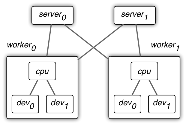
- On the first layer, data are synchronized over multiple devices within a single worker machine. A device could be a GPU card, CPU, or other computational units. We often use sequential consistency model, also known as BSP, on this level.
- On the second layer, data are synchronize over multiple workers via server machines. We can either use a sequential consistency model for guaranteed convergence or an (partial)-asynchronous model for better system performance.
KVStore
MXNet implemented the two-level parameter server in class KVStore. We currently provide the following three types. Given the batch size b:
| kvstore type | #devices | #workers | #ex per device | #ex per update | max delay |
|---|---|---|---|---|---|
| local | k | 1 | b / k | b | 0 |
| dist_sync | k | n | b / k | b × n | 0 |
| dist_async | k | n | b / k | b | inf |
where the number of devices k used on a worker could vary for different workers. And
- number examples per update : for each update, the number of examples used to calculate the averaged gradients. Often the larger, the slower the convergence.
- number examples per device : the number of examples batched to one device each time. Often the larger, the better the performance.
- max delay : The maximal delay of the weight a worker can get. Given a worker, a delay d for weight w means when this worker uses w (to calculate the gradient), w have been already updated by d times on some other places. A larger delay often improves the performance, but may slows down the convergence.
Multiple devices on a single machine
KV store local synchronizes data over multiple devices on a single machine.
It gives the same results (e.g. model accuracy) as the single device case. But
comparing to the latter, assume there are k devices, then each device only
processes 1 / k examples each time (also consumes 1 / k device memory). We
often increase the batch size b for better system performance.
When using local, the system will automatically chooses one of the following
three types. Their differences are on where to average
the gradients over all devices, and where to update the weight.
They produce (almost) the same results, but may vary on speed.
local_update_cpu, gradients are first copied to main memory, next averaged on CPU, and then update the weight on CPU. It is suitable when the average size of weights are not large and there are a large number of weight. For example the google Inception network.local_allreduce_cpuis similar tolocal_update_cpuexcept that the averaged gradients are copied back to the devices, and then weights are updated on devices. It is faster than 1 when the weight size is large so we can use the device to accelerate the computation (but we increase the workload by k times). Examples are AlexNet on imagenet.local_allreduce_deviceis similar tolocal_allreduce_cpuexcept that the gradient are averaged on a chosen device. It may take advantage of the possible device-to-device communication, and may accelerate the averaging step. It is faster than 2 when the gradients are huge. But it requires more device memory.
Multiple machines
Both dist_async and dist_sync can handle the multiple machines
situation. But they are different on both semantic and performance.
dist_sync: the gradients are first averaged on the servers, and then send to back to workers for updating the weight. It is similar tolocalandupdate_on_kvstore=falseif we treat a machine as a device. It guarantees almost identical convergence with the single machine single device situation if reduces the batch size to b / n. However, it requires synchronization between all workers, and therefore may harm the system performance.dist_async: the gradient is sent to the servers, and the weight is updated there. The weights a worker has may be stale. This loose data consistency model reduces the machine synchronization cost and therefore could improve the system performance. But it may harm the convergence speed.