
Design Efficient Deep Learning Data Loading Module
Data loading is an important part of the machine learning system, especially when the data is huge and do not fit into memory. The general design goal of data loading module is to achieve more efficient data loading, less effort on data preparation, clean and flexible interface.
This tutorial will be organized as follows: in IO Design Insight section, we introduce some insights and guidelines in our data loading design; in Data Format section, we introduce our solution using dmlc-core’s binary recordIO implementation; in Data Loading section, we introduce our method to hide IO cost by utilizing the Threadediter provided by dmlc-core; in the Interface Design section, we will show you the simple way to construct a MXNet data iterator in a few lines of python; in the Future Extension part, we discuss how to make data loading more flexible to support more learning tasks.
We will cover the following key requirements, in detail in the later part of sections.
List of Key Requirements
- Small file size.
- Allow parallel(distributed) packing of data.
- Fast data loading and online augmentation.
- Allow quick read arbitrary parts in distributed setting.
Design Insight
IO design usually involves two kinds of work: data preparation and data loading. Data preparation usually influences the time consuming offline, while data loading influences the online performance. In this section, we will introduce our insight of IO design involving the two phases.
Data Preparation
Data preparation is to pack the data into certain format for later processing. When the data is huge, i.e. full ImageNet, this process may be time-consuming. Since that, there’re several things we need to pay attention:
- Pack the dataset into small numbers of files. A dataset may contain millions of data instances. Packed data distributes easily from machine to machine;
- Do the packing once. No repacking is needed when the running setting has been changed (usually means the number of running machines);
- Process the packing in parallel to save time;
- Access to arbitrary parts easily. This is crucial for distributed machine learning when data parallelism is introduced. Things may get tricky when the data has been packed into several physical data files. The desired behavior could be: the packed data can be logically partite into arbitrary numbers of partitions, no matter how many physical data files there are. For example, we pack 1000 images into 4 physical files, each contains 250 images. Then we use 10 machines to training DNN, we should be able to load approximately 100 images per machine. Some machine may need images from different physical files.
Data Loading
Data loading is to load the packed data into RAM. One ultimate goal is to load as quickly as possible. Thus there’re several things we need to pay attention:
- Continuous reading. This is to avoid arbitrary reading from disk;
- Reduce the bytes to be loaded. This can be achieved by storing the data instance in a compact way, e.g. save the image in JPEG format;
- Load and train in different threads. This is to hide the loading time cost;
- RAM saving. We don’t want to load the whole file into the RAM if the packed file is huge.
Data Format
Since the training of deep neural network always involves huge amount of data, the format we choose should works efficient and convenient in such scenario.
To achieve the goals described in insight, we need to pack binary data into a splitable format. In MXNet, we use binary recordIO format implemented in dmlc-core as our basic data saving format.
Binary Record
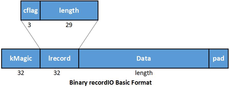 In binary recordIO, each data instance is stored as a record. kMagic is a Magic Number indicating the start of a record. Lrecord encodes length and continue flat.
In lrecord,
In binary recordIO, each data instance is stored as a record. kMagic is a Magic Number indicating the start of a record. Lrecord encodes length and continue flat.
In lrecord,
- cflag == 0: this is a complete record;
- cflag == 1: start of a multiple-rec;
- cflag == 2: middle of multiple-rec;
- cflag == 3: end of multiple-rec.
Data is the space to save data content. Pad is simply a padding space to make record align to 4 bytes.
After packing, each file contains multiple records. Loading can be continues. This avoids the low performance of random reading from disk.
One great advantage of storing data as record is each record can vary in length. This allow us to save data in a more compact way if compact algorithm is available for a certain kind of data. For example, we can use JPEG format to save image data. The packed data will be much smaller compared with storing in RGB value. We can take ImageNet_1K dataset as an example, if we store the data in 3 * 256 * 256 raw rgb value, the dataset may occupy more than 200G, while if we stored the data after compacting into JPEG, it only occupies about 35G disk space. It may greatly reduce the cost of reading disk.
Here’s an example of Image binary recordIO:
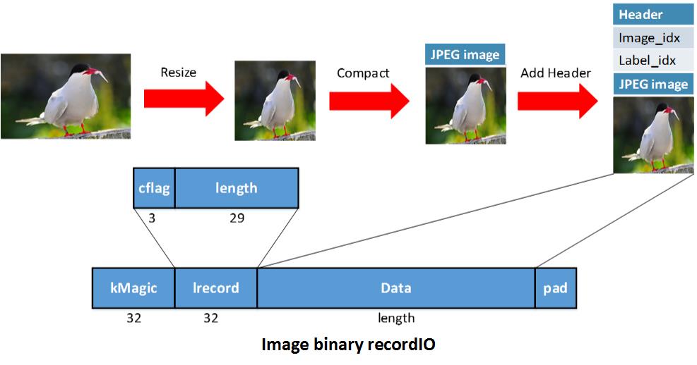 We first resize the image into 256 * 256, then compact it into JPEG format, after that we save the header which indicates the index and label for that image to construct the Data field of a record. Then pack several images together into a file.
Access Arbitrary Parts Of Data
The desired behavior of data loading could be: the packed data can be logically sliced into arbitrary numbers of partitions, no matter how many physical packed data files there are.
Since binary recordIO can easily locate the start and end of a record using the Magic Number, we can achieve the above goal using the InputSplit functionality provided by dmlc-core.
InputSplit takes the following parameters:
- FileSystem *filesys: dmlc-core encapsulate the IO operations for different filesystems, like hdfs, s3, local. User don’t need to worry about the difference between filesystems any more;
- Char *uri: the uri of files. Note that it could be a list of files, for we may pack the data into several physical parts. File uris are separated by ‘;’.
- Unsigned nsplit: the number of logical splits. Nsplit could be different from the number of physical file parts;
- Unsigned rank: which split to load in this process;
The splitting process is demonstrated below:
- Statist the file size of each physical parts. Each file contains several records;
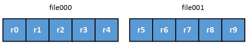
- Approximately partite according to file size. Note that the boundary of each part may locate in the middle of a record;
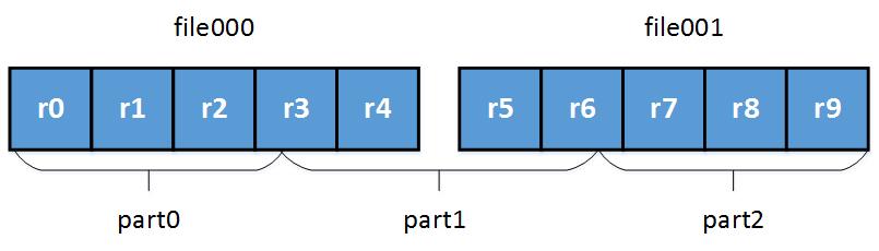
- Seek the beginning of records to avoid incomplete records to finish partition;
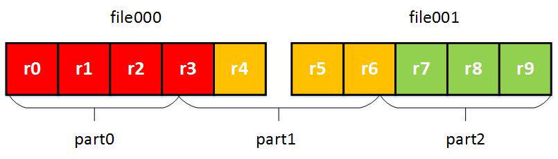
By conducting the above operations, we now identify the records belong to each part, and the physical data files needed by each logical part. InputSplit greatly reduce the difficulty of data parallelism, where each process only read part of the data.
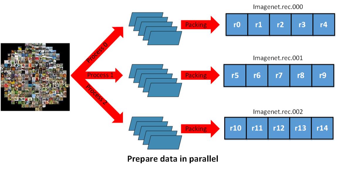
Since logical partition doesn’t rely on the number of physical data files, we can process huge dataset like ImageNet_22K in parallel easily as illustrated below. We don’t need to consider distributed loading issue at the preparation time, just select the most efficient physical file number according to the dataset size and the computing resources you have.
Data Loading and Preprocessing
When the speed of loading and preprocessing can’t catch up with the speed of training or evaluation, IO will become the bottleneck of the whole system. In this section, we will introduce our tricks to pursuit the ultimate efficiency to load and preprocess data packed in binary recordIO format. In our ImageNet practice, we can achieve the IO speed of 3000 images/s with normal HDD.
Loading and preprocessing on the fly
When training deep neural networks, we sometimes can only load and preprocess the data along with training because of the following reasons:
- The whole size of the dataset exceed the RAM size, we can’t load them in advance;
- The preprocessing pipeline may produce different output for the same data at different epoch if we would like to introduce randomness in training;
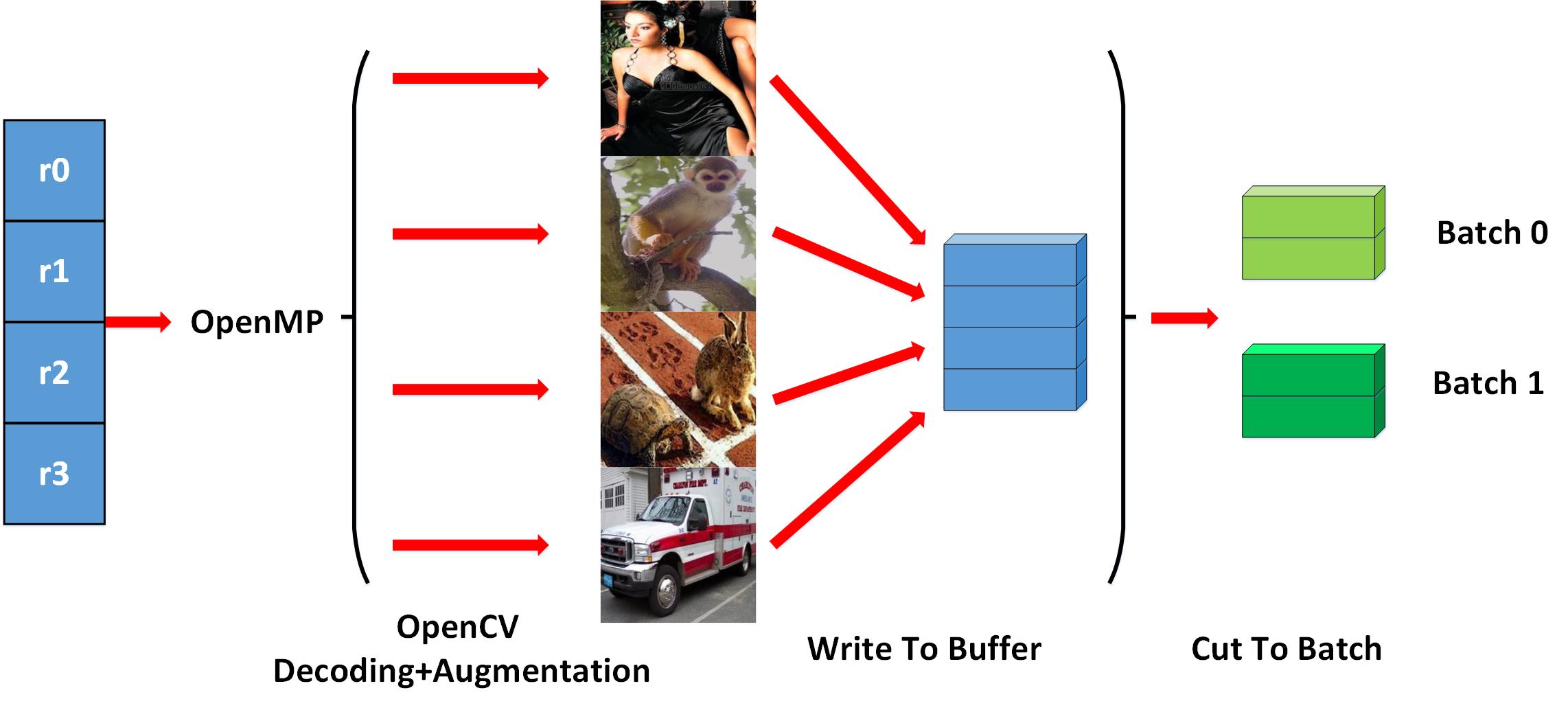
To achieve the goal of ultimate efficiency, multi-thread technic is introduced in the related procedures. We take imagenet training as an example, after loading a bunch of image records, we can start multiple threads to do the image decoding and image augmentation , as illustrated below:
Hide IO Cost Using Threadediter
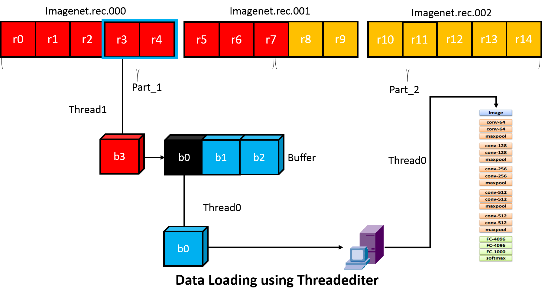
One way to hide IO cost is to prefetch the data for next batch on a stand-alone thread, while the main thread conducting feed-forward and backward. In order to support more complicated training schemas, MXNet provide a more general IO processing pipeline using threadediter provided by dmlc-core.
The key of threadediter is to start a stand-alone thread acts like a data provider, while the main thread acts like data consumer as illustrated below.
Threadediter will maintain a buffer of a certain size and automatically fill the buffer if it’s not full. And after the consumer finish consuming part of the data in the buffer, threadediter will reuse the space to save the next part of data.
MXNet IO Python Interface
We make the IO object as an iterator in numpy. By achieving that, user can easily access to the data using a for-loop or calling next() function. Defining a data iterator is very similar to define a symbolic operator in MXNet.
The following code gives an example of creating a Cifar data iterator.
dataiter = mx.io.ImageRecordIter(
    # Dataset Parameter, indicating the data file, please check the data is already there
    path_imgrec="data/cifar/train.rec",
    # Dataset Parameter, indicating the image size after preprocessing
    data_shape=(3,28,28),
    # Batch Parameter, tells how many images in a batch
    batch_size=100,
    # Augmentation Parameter, when offers mean_img, each image will substract the mean value at each pixel
    mean_img="data/cifar/cifar10_mean.bin",
    # Augmentation Parameter, randomly crop a patch of the data_shape from the original image
    rand_crop=True,
    # Augmentation Parameter, randomly mirror the image horizontally
    rand_mirror=True,
    # Augmentation Parameter, randomly shuffle the data
    shuffle=False,
    # Backend Parameter, preprocessing thread number
    preprocess_threads=4,
    # Backend Parameter, prefetch buffer size
    prefetch_buffer=1)
Generally to create a data iterator, you need to provide five kinds of parameters:
- Dataset Param gives the basic information for the dataset, e.g. file path, input shape.
- Batch Param gives the information to form a batch, e.g. batch size.
- Augmentation Param tells which augmentation operations (e.g. crop, mirror) should be taken on an input image.
- Backend Param controls the behavior of the backend threads to hide data loading cost.
- Auxiliary Param provides options to help checking and debugging.
Usually, Dataset Param and Batch Param MUST be given, otherwise data batch can’t be created. Other parameters can be given according to algorithm and performance need, or just use the default value we set for you.
Ideally we should separate the MX Data IO into modules, some of which might be useful to expose to users: Efficient prefetcher: allow the user to write a data loader that reads their customized binary format, and automatically enjoy multi-thread prefetcher support Data transformer: image random cropping, mirroring, etc. should be quite useful to allow the users to use those tools, or plug in their own customized transformers (maybe they want to add some specific kind of coherent random noise to data, etc.)
Future Extension
The data IO for some common applications that we might want to keep in mind: Image Segmentation, Object localization, Speech recognition. More detail will be provided when such applications have been running on MXNet.
Contribution to this Note
This note is part of our effort to open-source system design notes for deep learning libraries. You are more welcomed to contribute to this Note, by submitting a pull request.